Stochastic battery optimization using SDDP.jl

In a previous note I looked at optimizing the dispatch of a battery with stochastic price information by hand. Here, I will use a Julia package, SDDP.jl , that implements stochastic dual dynamic programming to do the same.

Here I will just use the library SDDP.jl and later dig into how SDDP works in detail.

Model assumptions

With $e_t$ the SoC of the battery in MWh entering stage $t$ and $p_t$ the grid-side battery power in MW. Grid-side means: $p_t > 0$ the battery discharges and vice versa.

To keep things simple, for a one hour settlement period and 100% efficiency:

e_{t+1} = e_t - p_t

Since $\Delta t = 1$ h, I suppress $\Delta t$ below. More generally:

e_{t+1} = e_t - p_t \Delta t

and stage P&L is $\pi_t p_t \Delta t$ .

Let’s go through this for a 1 MW / 1 MWh battery:

e_t \in [0,1], \qquad p_t \in [-1,1].

State (SoC) transitions are therefore:

e_{t+1} = e_t - p_t.

Across all stages we want to maximize our expected P&L:

\max \mathbb{E} \left[ \sum_t \pi_t p_t \right].

At each stage, the current price is observed before dispatch is chosen. Prices are independent across stages. There is no terminal energy requirement or value assigned to energy left after stage 3.

Julia implementation

Let us implement this in Julia using JuMP and SDDP.jl macros:

using SDDP
using JuMP
using HiGHS
using Printf

prices = [
    [40.0],
    [20.0, 80.0],
    [10.0, 100.0],
]

probabilities = [
    [1.0],
    [0.5, 0.5],
    [0.5, 0.5],
]

function build_stage(subproblem, stage)
    @variable(subproblem, 0 <= soc <= 1, SDDP.State, initial_value = 0.5)
    @variable(subproblem, -1 <= p <= 1)
    @constraint(subproblem, soc.out == soc.in - p)

    function set_stage_price(revealed_stage_price)
        @stageobjective(subproblem, revealed_stage_price * p)
    end

    SDDP.parameterize(
        set_stage_price,
        subproblem,
        prices[stage],
        probabilities[stage],
    )
end

model = SDDP.LinearPolicyGraph(
    build_stage;
    stages = 3,
    sense = :Max,
    upper_bound = 220.0,
    optimizer = HiGHS.Optimizer,
)

SDDP.train(
    model;
    iteration_limit = 50,
    log_frequency = 10,
)

bound = SDDP.calculate_bound(model)
println("Upper bound on expected P&L: ", bound)

Checking the policy

Here I implement the same price scenarios and 50/50 scenario probabilities I used in my earlier note. Let me run the code and see what SDDP.jl returns:

-------------------------------------------------------------------
         SDDP.jl (c) Oscar Dowson and contributors, 2017-26
-------------------------------------------------------------------
problem
  nodes           : 3
  state variables : 1
  scenarios       : 4.00000e+00
  existing cuts   : false
options
  solver          : serial mode
  risk measure    : SDDP.Expectation()
  sampling scheme : SDDP.InSampleMonteCarlo
subproblem structure
  VariableRef                             : [4, 4]
  AffExpr in MOI.EqualTo{Float64}         : [1, 1]
  VariableRef in MOI.GreaterThan{Float64} : [2, 3]
  VariableRef in MOI.LessThan{Float64}    : [3, 3]
numerical stability report
  matrix range     [1e+00, 1e+00]
  objective range  [1e+00, 1e+02]
  bounds range     [1e+00, 2e+02]
  rhs range        [0e+00, 0e+00]
-------------------------------------------------------------------
 iteration    simulation      bound        time (s)     solves  pid
-------------------------------------------------------------------
        10  -1.000000e+01  4.750000e+01  2.147027e+00        80   1
        20   6.000000e+01  4.750000e+01  2.204524e+00       160   1
        30   8.000000e+01  4.750000e+01  2.223780e+00       240   1
        40   8.000000e+01  4.750000e+01  2.236254e+00       320   1
        50  -1.000000e+01  4.750000e+01  2.248431e+00       400   1
-------------------------------------------------------------------
status         : iteration_limit
total time (s) : 2.248431e+00
total solves   : 400
best bound     :  4.750000e+01
numeric issues : 0
-------------------------------------------------------------------

Upper bound on expected P&L: 47.5

Revealed prices [40.0, 20.0, 10.0]       | Total P&L:   -10.00 Euro
Revealed prices [40.0, 80.0, 10.0]       | Total P&L:    60.00 Euro
Revealed prices [40.0, 20.0, 100.0]      | Total P&L:    80.00 Euro
Revealed prices [40.0, 80.0, 100.0]      | Total P&L:    60.00 Euro

Average policy P&L:    47.50 Euro
SDDP upper bound:      47.50 Euro
Optimality gap:         0.00 Euro

What we can see is that SDDP.jl gives us the same expected value to go / maximal expected value we can achieve across the entire optimization horizon:

V_1(0.5,40)=47.5\text{ Euro} = \text{ best SDDP bound}

What SDDP.jl does is learn a policy that we can use to unroll the different possible decision paths with. Doing so reveals the following decision tree:

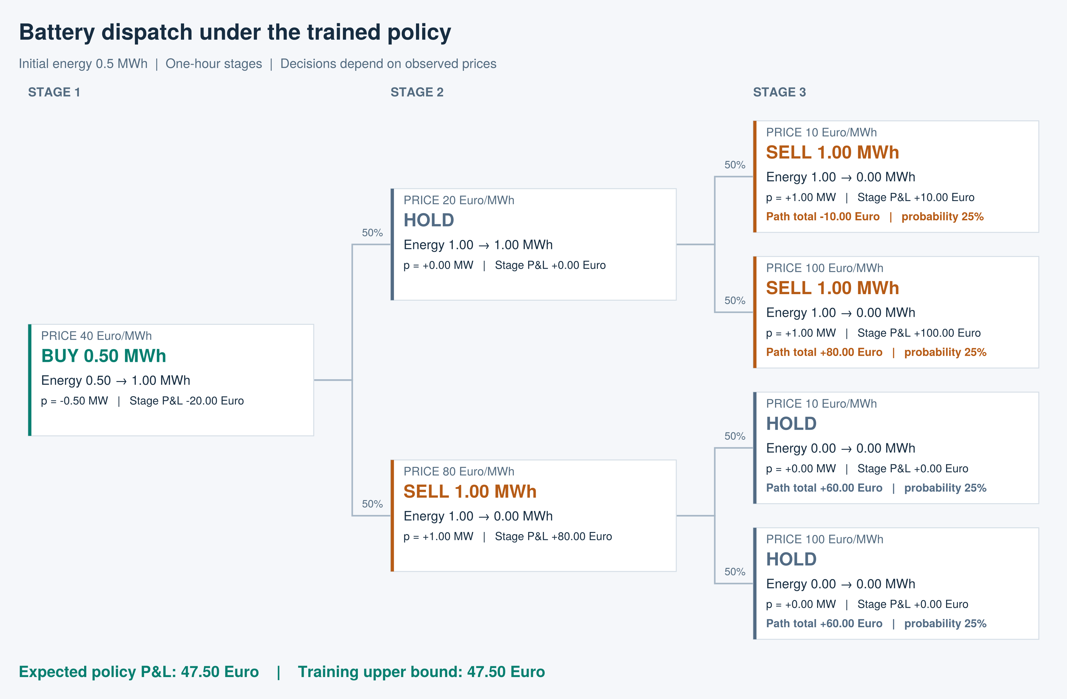
Decision tree for the equal-probability scenario.

Evaluating the trained policy on all four paths gives an expected P&L of €47.50. This matches the SDDP upper bound, so the policy is optimal for this model:

.25 \cdot (-10 \text{ Euro} + 80 \text{ Euro} + 60 \text{ Euro} + 60 \text{ Euro}) = 47.5 \text{ Euro} = V_1(0.5,40)

Changing the scenario probabilities

With this SDDP.jl implementation we can also play a bit with the scenarios. Let me change the scenario probabilities for stage 2 to express a greater conviction in a stage 2 low price scenario:

prices = [
    [40.0],
    [20.0, 80.0],
    [10.0, 100.0],
]

probabilities = [
    [1.0],
    [0.7, 0.3],  # I changed this from [0.5, 0.5]
    [0.5, 0.5],
]

Now our decision tree looks as follows:

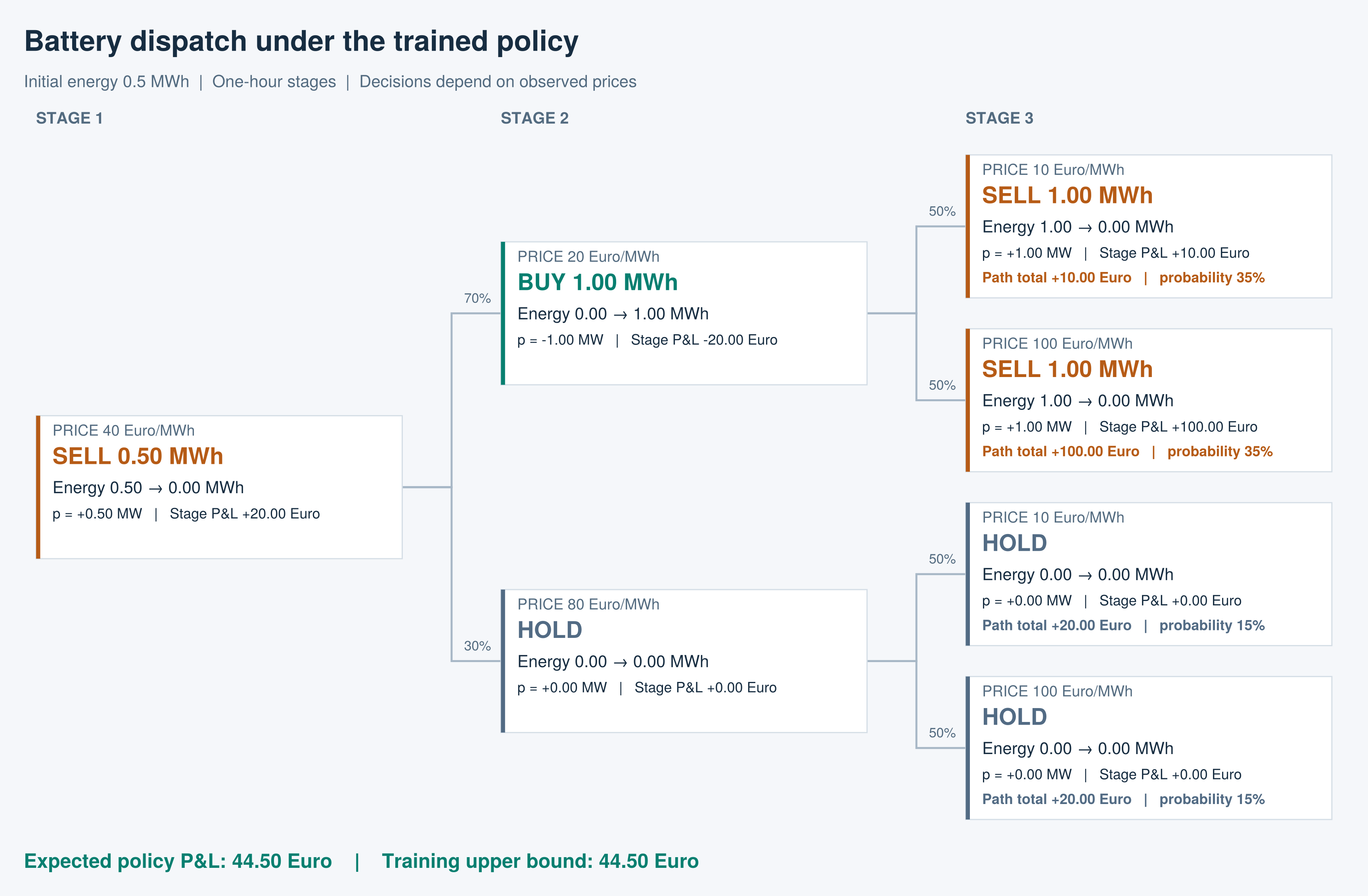
Decision tree with a higher probability of the low-price second stage.

We can see that the expected P&L has dropped to $V_1(0.5,40) = 44.5 \text{ Euro}$ however we now have a 35% chance of making 100 Euro in total.

I think this is a great starting point for digging further into how SDDP works and how SDDP.jl implements it.

Model assumptions#

Julia implementation#

Checking the policy#

Changing the scenario probabilities#

Model assumptions

Julia implementation

Checking the policy

Changing the scenario probabilities